IO and Visualization
Start by dowloading Teapot dome 3D open source dataset.
Next we need to find information about spatial refernce used in downloaded data.
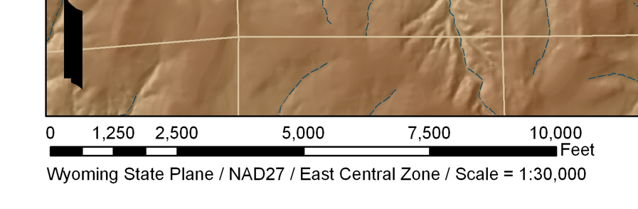
For that go to DataSets/GIS/CD files and open NPR3_BASEMAP.jpg that shows the survey on the relief map.
In the lower left corner there is a spatial reference and units:
Application settings
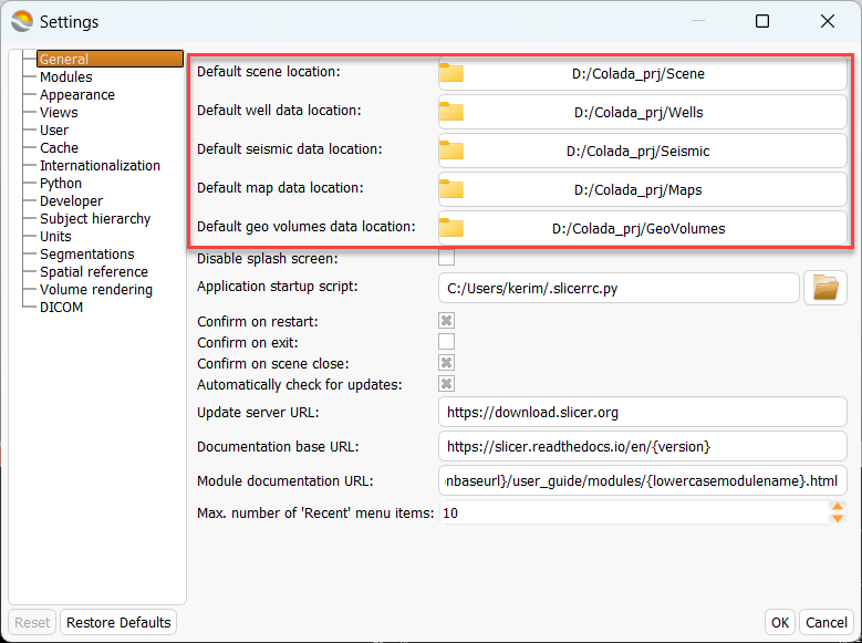
In Colada application settings (Toolbar menu->Edit->Application Settings) General panel set default directories for the data.
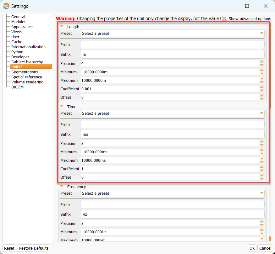
In the Units panel set preffered length and temporal units. In my case those are meter and millisecond.
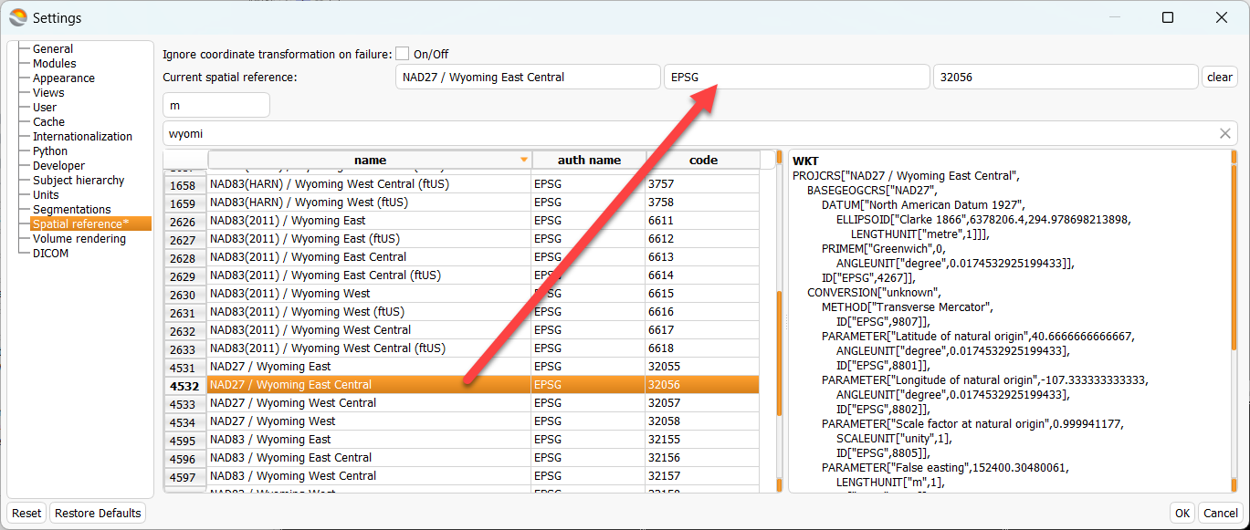
Then go to the spatial reference panel and find the appropriate one.
It seems that NAD27 / Wyoming East Central (EPSG:32056) is the right choice.
Set it using drag&drop.
Read SEGY
SEGY is represented by 3D STACK (Seismic/CD files/3D_Seismic/filt_mig.sgy) and bunch of 2D STACK (DataSets/Seismic/CD files/2D_Seismic) datasets.
In Colada SEGY STACK may be read as Geo Volume or as Seismic object. We will read it as Geo Volume first and then as Seismic.
Read SEGY as Geo Volume
To open Geo Volume SEGY reader right-click on Geo Volume tree Import->SEGY STACK.
Add SEGY files from DataSets/Seismic/CD files/2D_Seismic/NormalizedMigrated_segy/ and DataSets/Seismic/CD files/3D_Seismic/ directories.
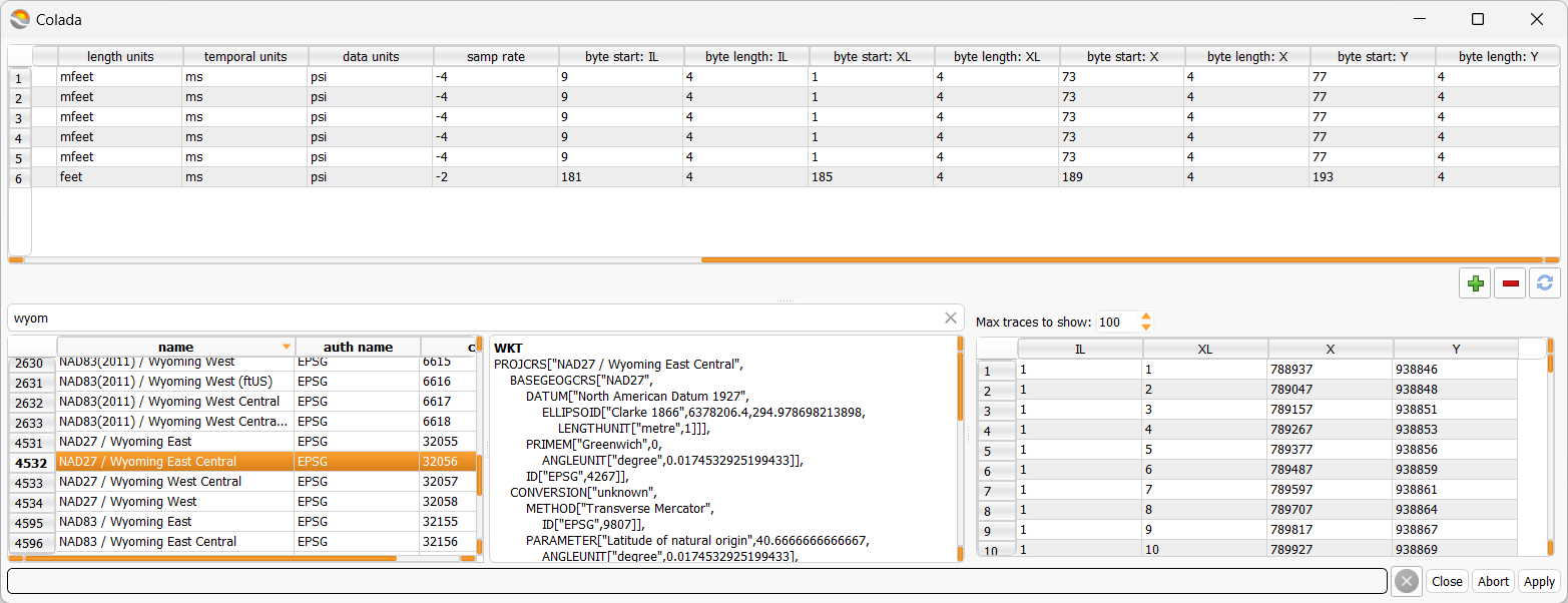
Before reading SEGY don’t forget to check trace headers.
For Teapot Dome the correct header offsets for INLINE, XLINE and X, Y are shown in the picture.
Warning
Geo Volume is a regular grid that can be represented by origin, orientation and spacings along each axis.
SEGY stack data may not strictly follow this. In this case XY plane will be broken and in practice the user must be confident that the SEGY is represented as a cube or flat with regular spacings.
There are few things that should be explained.
First of all each geo-object has attribute Domain.
Possible values are: TWT (Two Way Traveltime), OWT (One Way Traveltime), TVD (True Vertical Depth), TVDSS (True Vertical Depth Sub-Sea).
CRS (Coordinate Seference System or Spatial Reference System) highly desirable for every geo-object.
Length units, Temporal units necessary for all geo-objects. Uusually they are needed to define coordinates.
Data units necessary for some geo-objects like Map if it is in TWT/OWT domain.
Or for Geo Volume if it is going to be used in wave-modeling as velocity model for example.
Data units defines units of the data, for example for a Map object it defines units of surface values.
Or for Geo Volume it defines units of each scalar value of data (pressure for example or particle displacement).
To be confident that your units are convertable one may use the web service.
Geo Volume visualization
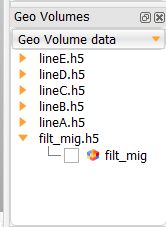
After data is read it should appear in the Geo Volume tree.
As Geo Volume may be pretty big and not all the time the user wants to load oll data to the memory, after clicking on the checkbox the module will be switched to GeoVolumes where one can select a subset of the data to load.
When the data is loaded new item will appear in Subject Hierarchy window. To visualize Geo Volume one may click on eye picture like shown in the picture.

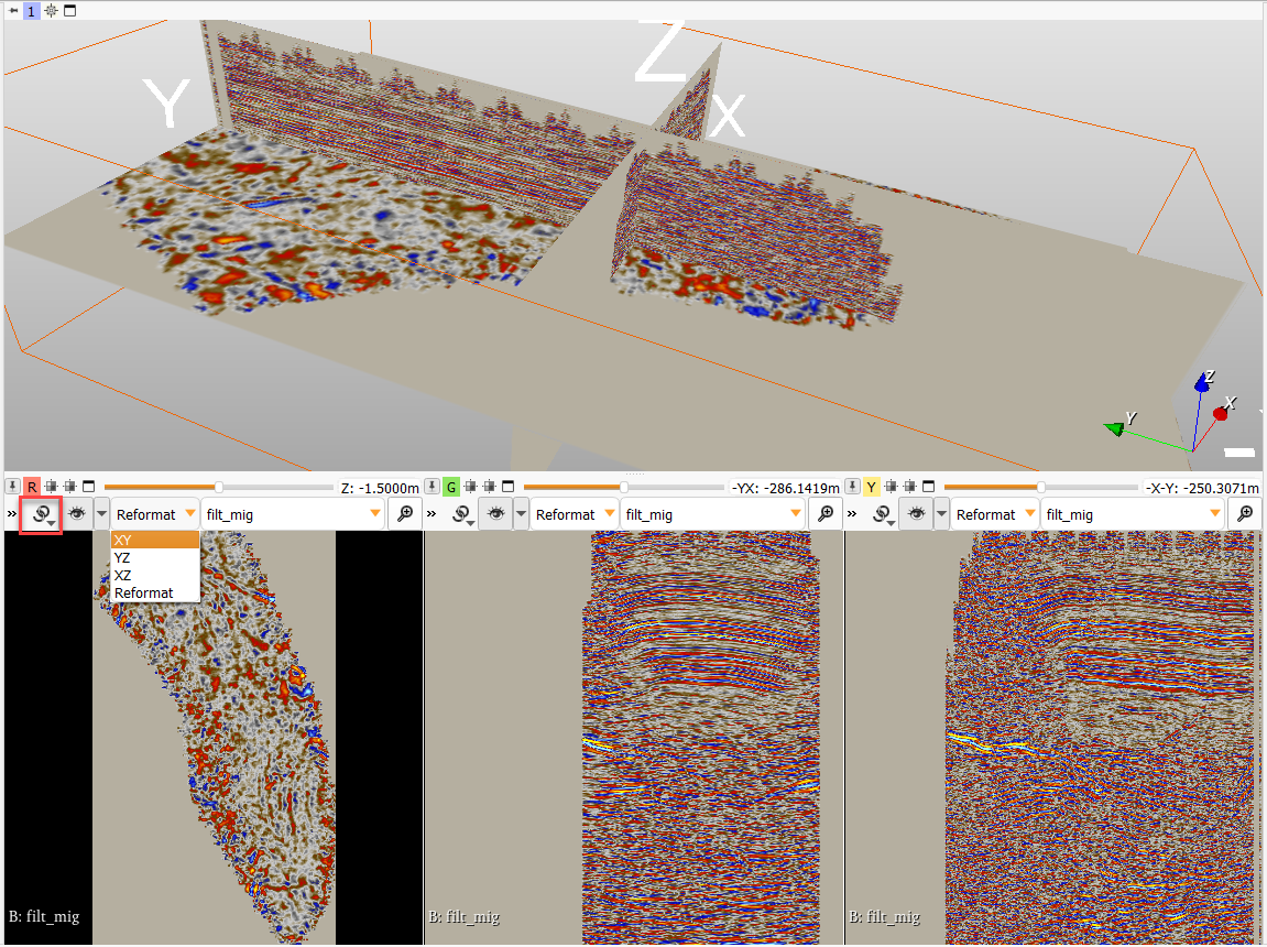
Geo Volume should be visualized.
By default Slice Views are synchronized. One can disable taht by clicking on the chain button.
To see axes in Slice View one should change the preset to one of the following: XY, YZ, XZ.
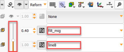
Further one can visualize two volumes one upon another. To do that there is a place for background and foreground volumes. Place 2D as background and 3D cuba as foreground. Then using slicer change the opacty to see how these two objects relates.
Another way to visualize the data is to drag&drop the selected object to the scene. In this case an object will be rendered as Volume.
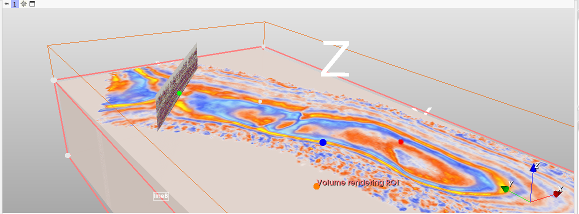
Rendered Volume is controlled in Volume Rendering module.
Volume module is for usual representation using Slices.
Check these modules to see how you can customize the visualization.
Read SEGY as Seismic
To read SEGY as Seismic right click on Seismic treeview to invoke menu Import->SEGY.
Add the same files as we have read with Geo Volume reader.
Carefully set all the parameters. it is important to set survey type (2D/3D), data type (stack/prestack), domain, units ,sampling rate.
Note
Colada uses Z values decreases downwards. That means when reading usual SEGY file as Seismic one need to set negative sampling rate.

Provided SEGY files have mixed trace headers. INLINE/XLINE are either missing or switched with CDP_X/CDP_Y (for 3D).
CDP_X/CDP_Y are switched with SRCX/SRCY (for 2D).
To fix that there is table in the middle of the window. The point is to set the correct trace header names for all trace header offsets. If you do this correctly then all modified items in the table will be colored by green color. Be sure there is no red colored boxes.
Seismic visualization
When working with Seismic it usually requires some kind of a sorting. As Colada provides means to work with STACK as well as with STACK seismic the user should be familiar with seismic sorting.
Colada doesn’t resort data itself but it rather writes trace indices for every primary key value (pKey).
For example if we want to get INLINE->XLINE then we need to prepare sorting for INLINE as it is a primary key.
The sorting is efficient when the number of unique values a lot less of the amount of traces.
Thus sorting for CDP/SP/INLINE/XLINE etc are pretty effective.
So click on the checkbox in the Seismic Tree and Seismic module appear.
Expand sorting tab and add INLINE sorting.
Then X/Y coord headers as CDP_X/CDP_Y and load it.
Seismic may be loaded as:
Volume (rectangular grid, 3D)
Volumetric mesh (unstructured grid, 3D)
Surface (2D)
Volume uses interpolation if the original data has random XY coordinates.
Volumetric mesh use data as is but it requires about four times more RAM tan Volume.
Surface is for 2D selected data.
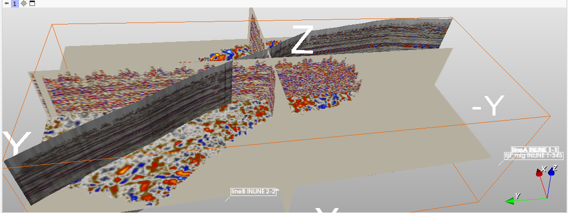
For example we can load the same 2D seismic lineA as Volume and then as Surface and see the difference.

In the same way we can visualize 3D seismic as volume.
Volume visualization is controlled by Volumes and Volume Rendering modules.
Surface and Volumetric mesh is controlled by Models module.
All the loaded data is displayed in Data module.
Try to play with it.
Read Well data
In DataSets/Well Log/CD Files there are DirectionalSurveys_020910.xlsx, TeapotDomeWellHeaders02-09-10.xlsx, TeapotDomeFormationLogTops.xlsx.
This is not a standardized file format.
To read it we will use Python.
We can read it using Pandas package for example.
Or preinstall desired package using slicer.util.pip_install("my_package") and use it.
But as I already did it using csv we will export Excel to csv comma delimited file and then process it.
Note
To run the Python code one either need to copy-paste it to the Interpreter or save it as script and Ctrl + g. Or from command line ./Colada --python-script <path-to-file>
Read Well Heads
This snippet reads well heads from comma delimited TeapotDomeWellHeaders02-09-10.csv file (don’t forget to change readfile path at the bottom).
from PythonQt import *
from qColadaAppPythonQt import *
from h5geopy import h5geo
import numpy as np
import csv


def readTeapotWellHeads(readfile: str, savefile: str):
  def is_float(element) -> bool:
    try:
      float(element)
      return True
    except ValueError:
      return False
  # set parameters for the newly created well
  p_w = h5geo.H5WellParam()
  p_w.spatialReference = h5geo.sr.getAuthName() + ':' + h5geo.sr.getAuthCode()
  p_w.lengthUnits = 'feet'
  p_w.temporalUnits = 'ms'
  p_w.angularUnits = 'degree'
  # set parameters for the newly created devcurve
  p_d = h5geo.H5DevCurveParam()
  p_d.spatialReference = h5geo.sr.getAuthName() + ':' + h5geo.sr.getAuthCode()
  p_d.lengthUnits = 'feet'
  p_d.temporalUnits = 'ms'
  p_d.angularUnits = 'degree'
  p_d.chunkSize = 1 # we set only signle row to curve. Chunking affects on the datasize
  wellname = ''
  kb = 0
  head_xy = np.zeros(2, order='F')
  # create hdf5 well container
  h5wellCnt = h5geo.createWellContainerByName(savefile, h5geo.CreationType.CREATE_OR_OVERWRITE)
  if not h5wellCnt:
    raise ValueError(f"Unable to create or overwrite Well Container: {savefile}")
  with open(readfile,) as csvfile:
    QtGui.QApplication.setOverrideCursor(QtCore.Qt.BusyCursor)
    reader = csv.reader(csvfile, dialect='excel')
    for line in reader:
      if reader.line_num < 3:
        continue
      if len(line) < 11 or not is_float(line[4]) or not is_float(line[5]) or not is_float(line[9]):
        continue
      if 'kb' not in line[10].lower():
        continue
      p_w.uwi = line[0][5:10]  # info https://en.wikipedia.org/wiki/API_well_number
      wellname = line[3].replace('/', '') # symbol `/` creates new group in hdf5
      head_xy[0] = float(line[5])
      head_xy[1] = float(line[4])
      kb = float(line[9])
      # create well (skip if fail)
      h5well = h5wellCnt.createWell(wellname, p_w, h5geo.CreationType.CREATE_OR_OVERWRITE)
      if not h5well:
        continue
      h5well.setHeadCoord(head_xy)
      h5well.setKB(kb)
      # create devcurve (skip if fail)
      h5devCurve = h5well.createDevCurve('vertical trajectory', p_d, h5geo.CreationType.CREATE)
      if not h5devCurve or not is_float(line[8]):
        continue
      md = np.zeros(2)
      md[1] = float(line[8])  # assuming that well is vertical then MD = TVD
      azim = np.zeros(2)
      incl = np.zeros(2)
      h5devCurve.writeMD(np.asfortranarray(md, dtype=float))
      h5devCurve.writeAZIM(np.asfortranarray(azim, dtype=float))
      h5devCurve.writeINCL(np.asfortranarray(incl, dtype=float))
      h5devCurve.updateTvdDxDy()
      if not h5well.openActiveDevCurve():
        h5devCurve.setActive()
    QtGui.QApplication.restoreOverrideCursor()
    print(f"Well headers file read to: {savefile}")

# ===============================
# CHANGE THE PATH TO THE CSV FILE
# ===============================
readfile = r'E:\\Teapot Dome\\DataSets\\Well Log\\CD Files\\TeapotDomeWellHeaders02-09-10.csv'
savefile = Util.defaultWellDir() + "/wells.h5"


readTeapotWellHeads(readfile,savefile)
Read Deviations
Implemented deviation reader is based on format like those exported by Petrel.
In this example the format is Excel.
Export it to csv and run:
from PythonQt import *
from qColadaAppPythonQt import *
from h5geopy import h5geo
import numpy as np


def readTeapotDeviations(readfile: str, savefile: str):
  def is_float(element) -> bool:
    try:
      float(element)
      return True
    except ValueError:
      return False
  p_w = h5geo.H5WellParam()
  p_w.spatialReference = h5geo.sr.getAuthName() + ':' + h5geo.sr.getAuthCode()
  p_w.lengthUnits = 'feet'
  p_w.temporalUnits = 'ms'
  p_w.angularUnits = 'degree'
  p_d = h5geo.H5DevCurveParam()
  p_d.spatialReference = h5geo.sr.getAuthName() + ':' + h5geo.sr.getAuthCode()
  p_d.lengthUnits = 'feet'
  p_d.temporalUnits = 'ms'
  p_d.angularUnits = 'degree'
  p_d.chunkSize = 10
  h5wellCnt = h5geo.createWellContainerByName(savefile, h5geo.CreationType.OPEN_OR_CREATE)
  if not h5wellCnt:
    raise ValueError(f"Unable to open or create Well Container: {savefile}")
  h5well = None
  h5devCurve = None
  m = np.zeros([0,3])
  need_write = False
  dev_curve_name = None
  with open(readfile) as file:
    QtGui.QApplication.setOverrideCursor(QtCore.Qt.BusyCursor)
    for line in file:
      strlist = line.split()
      if len(strlist) > 1 and 'well' in strlist[0].lower():
        m = np.zeros([0,3])
        need_write = True
      elif (len(strlist) > 3 and is_float(strlist[1]) and
          is_float(strlist[2]) and is_float(strlist[3])):
        p_w.uwi = strlist[0][5:10]
        dev_curve_name = strlist[0][10:12]  # info https://en.wikipedia.org/wiki/API_well_number
        m = np.append(m, np.zeros([1,3]), axis=0)
        m[-1,0] = float(strlist[1]) # MD
        m[-1,1] = float(strlist[3]) # AZIMUTH
        m[-1,2] = float(strlist[2]) # INCLINATION
      elif len(strlist) < 1 and m.shape[0] > 0 and need_write:
        if not dev_curve_name or not p_w.uwi:
          continue
        # create well (skip if fail)
        h5well = h5wellCnt.openWellByUWI(p_w.uwi)
        if not h5well:
          continue
        h5devCurve = h5well.createDevCurve(dev_curve_name, p_d, h5geo.CreationType.OPEN_OR_CREATE)
        if not h5devCurve:
          continue
        h5devCurve.setActive()
        h5devCurve.writeMD(np.asfortranarray(m[:,0], dtype=float))
        h5devCurve.writeAZIM(np.asfortranarray(m[:,1], dtype=float))
        h5devCurve.writeINCL(np.asfortranarray(m[:,2], dtype=float))
        h5devCurve.updateTvdDxDy()
        need_write = False
    if need_write and dev_curve_name and p_w.uwi:
      h5well = h5wellCnt.openWellByUWI(p_w.uwi)
      if h5well:
        # create devcurve (skip if fail)
        h5devCurve = h5well.createDevCurve(dev_curve_name, p_d, h5geo.CreationType.OPEN_OR_CREATE)
        if h5devCurve:
          h5devCurve.setActive()
          h5well.setUWI(p_w.uwi)
          h5devCurve.writeMD(np.asfortranarray(m[:,0], dtype=float))
          h5devCurve.writeAZIM(np.asfortranarray(m[:,1], dtype=float))
          h5devCurve.writeINCL(np.asfortranarray(m[:,2], dtype=float))
          h5devCurve.updateTvdDxDy()
    QtGui.QApplication.restoreOverrideCursor()
    print(f"Dev file read to: {savefile}")

# ===============================
# CHANGE THE PATH TO THE CSV FILE
# ===============================
readfile = r'E:\\Teapot Dome\\DataSets\\Well Log\\CD Files\\DirectionalSurveys_020910.csv'
savefile = Util.defaultWellDir() + "/wells.h5"


readTeapotDeviations(readfile, savefile)
Read Well Tops
Once again export TeapotDomeFormationLogTops.xlsx to csv and run:
from PythonQt import *
from qColadaAppPythonQt import *
from h5geopy import h5geo
import numpy as np
import csv


def readTeapotWellTops(readfile: str, savefile: str):
  p_wt = h5geo.H5WellTopsParam()
  p_wt.nPoints = 1
  p_wt.chunkSize = 5
  p_wt.domain = h5geo.Domain.TVD
  p_wt.spatialReference = h5geo.sr.getAuthName() + ':' + h5geo.sr.getAuthCode()
  p_wt.lengthUnits = 'feet'
  data = {}
  wellname_old = ''
  wellname_new = ''
  h5wellCnt = h5geo.createWellContainerByName(savefile, h5geo.CreationType.OPEN)
  if not h5wellCnt:
    raise ValueError(f"Unable to open Well Container: {savefile}")
  with open(readfile,) as csvfile:
    QtGui.QApplication.setOverrideCursor(QtCore.Qt.BusyCursor)
    reader = csv.reader(csvfile, dialect='excel')
    for line in reader:
      if reader.line_num < 2 or len(line) != 4:
        continue
      if reader.line_num == 2:
        wellname_old = line[1]
      else:
        wellname_old = wellname_new
      wellname_new = line[1]
      if wellname_old != wellname_new:
        h5well = h5wellCnt.openWell(wellname_old)
        if not h5well:
          continue
        h5welltops = h5well.createWellTops(p_wt, h5geo.CreationType.OPEN_OR_CREATE)
        if not h5welltops:
          continue
        p_wt.nPoints = len(data)
        p_wt.chunkSize = len(data)
        h5welltops.writeData(data, 'feet')
      topsname = line[2]
      md = float(line[3])
      data[topsname] = md
    QtGui.QApplication.restoreOverrideCursor()
    print(f"Well Tops file read to: {savefile}")

# ===============================
# CHANGE THE PATH TO THE CSV FILE
# ===============================
readfile = r'E:\\Teapot Dome\\DataSets\\Well Log\\CD Files\\TeapotDomeFormationLogTops.csv'
savefile = Util.defaultWellDir() + "/wells.h5"


readTeapotWellTops(readfile,savefile)
Read LAS
Fortunately LAS standardized format and thus there is graphical interface for reading it.
Right click on Well Tree and Import->LAS.
From DataSets/Well Log/CD Files/LAS_log_files/Deeper_LAS_files/ directory add LAS files to the reader.
Wait, this will take a while.
Change save to for the container used for reading well heads, well tops and deviations (/some/path/wells.h5).
Actively use copy&paste for that.
Probably it is worth to check on the box find well by UWI as well names and not always correct.
For that select the whole column and check on the box: this will cause all the column to be checked.
In the right table one can exclude/modify curves.
Reading LAS takes some time.

Well Visualization
After it is finished go to the Well treeview select some wells and check them.
If you are lucky wells appear in the scene.
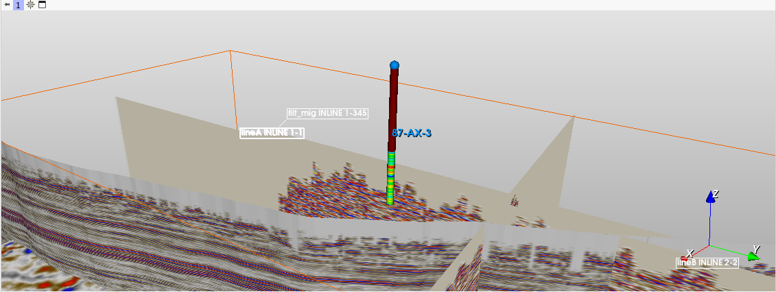
If not then choose 87-AX-3 it contains both trajectory and logs.
Go to the Wells module and select loaded well.
A number of deviations and logs should appear in the tables.
Load trajectory using 200 resampled points.
Then load CALD/CALD log.
The scene now should look like in the picture:
Then check on Variant Thickness and adjust radius and smooth.

Further customizations are done in Markups module.
Try to play with it.